Evaluating the Relationships between Muscle Oxygenation, Ventilation, and Lactate Thresholds

One of the projects I’ve been working on lately is a study comparing physiological breakpoints between ventilatory thresholds, lactate thresholds, and NIRS-derived deoxygenation breakpoints. I’ll cover all of these briefly as we go through the process. My objective is to help standardize the analysis of meaningful NIRS breakpoints, as has long been done for ventilation and lactate.

I feel like the sport science community is at the point right now where ‘expert evaluation’ of NIRS parameters is centralizing toward a common understanding and interpretation of signals. But by no means is there consensus yet on which NIRS parameters are the most relevant, or how best to analyze those parameters systematically.

To give my conclusion at the top, because I think it’s important to frame the conversation around thresholds and breakpoints: I think having a systematic approach to metabolic profiling is important, to define the rules that our brains are already using automatically to detect patterns in the data, in order to better understand the real (and differentiate the not-so-real) physiological relationships for an individual athlete. I think the next generation approach to metabolic profiling and training prescription will almost certainly not include breakpoint or threshold demarcations at all, and will use more flexible methods of describing continuous physiological response profiles in real-time.

That being said, we have to start somewhere with the precedent of established methods for determining common physiological responses and training prescription. So here is the current approach I’m using for breakpoint detection across lactate, ventilatory, and muscle oxygenation data. This is very much a work in progress, and I expect my approach will change!

---

Intermittent Progressive Cycling Assessment

The assessment protocol we are using is a ‘5-1’ intermittent multi-stage cycling test, with 5-minute stages at constant workloads and 1-minute rest periods between stages. We are starting at 1.0 W/kg and progressing by 0.5 W/kg per stage. We have a superfluous number of Moxy NIRS sensors on left and right muscles measuring muscle oxygenation, or saturation (SmO2). The subjects are breathing into a mask collecting pulmonary gas exchange (eg. VO2). And we are taking fingertip capillary lactate measurements at the end of each work stage.

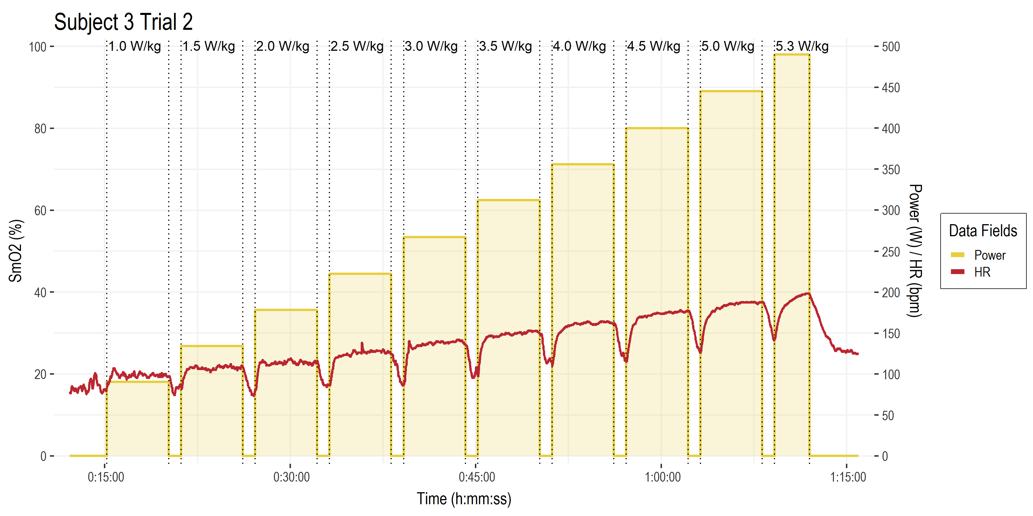
• The basic exercise protocol.
• Time on the x-axis.
• Power (W ) and heart rate (HR, bpm) both on the right y-axis. Gold bars are work stage power targets (W/kg along the top). Red line is HR.
• Not pictured are all the rest of the data channels from Moxy sensors, gas exchange parameters, blood lactate, etc.

Let’s start with blood lactate (BLa) since these methods are probably the most established for this kind of constant workload multi-stage assessment protocol.

---

Lactate Thresholds

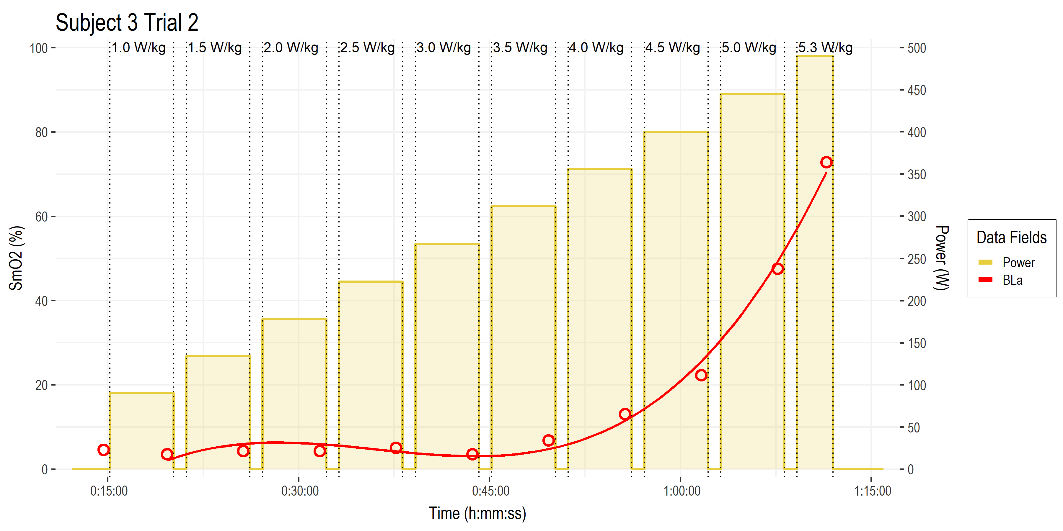
• Here are the time series data for blood lactate, in red. With each measurement point as the open circles, and a polynomial trendline plotted through those values.
• Time on the x-axis.
• BLa (mmol/L) is scaled from 0 to 20 mmol/L on the y-axis (divide the SmO2 y-axis on the left side by 5 to go from 0 to 20)

To begin analyzing BLa breakpoints we want to transform the plot from time to power on the x-axis. So that when we model regression lines of y (BLa) on x (power), we will get a power number along a continuous range from the model prediction, rather than being constrained to the discrete 0.5 W/kg jumps of each work interval.

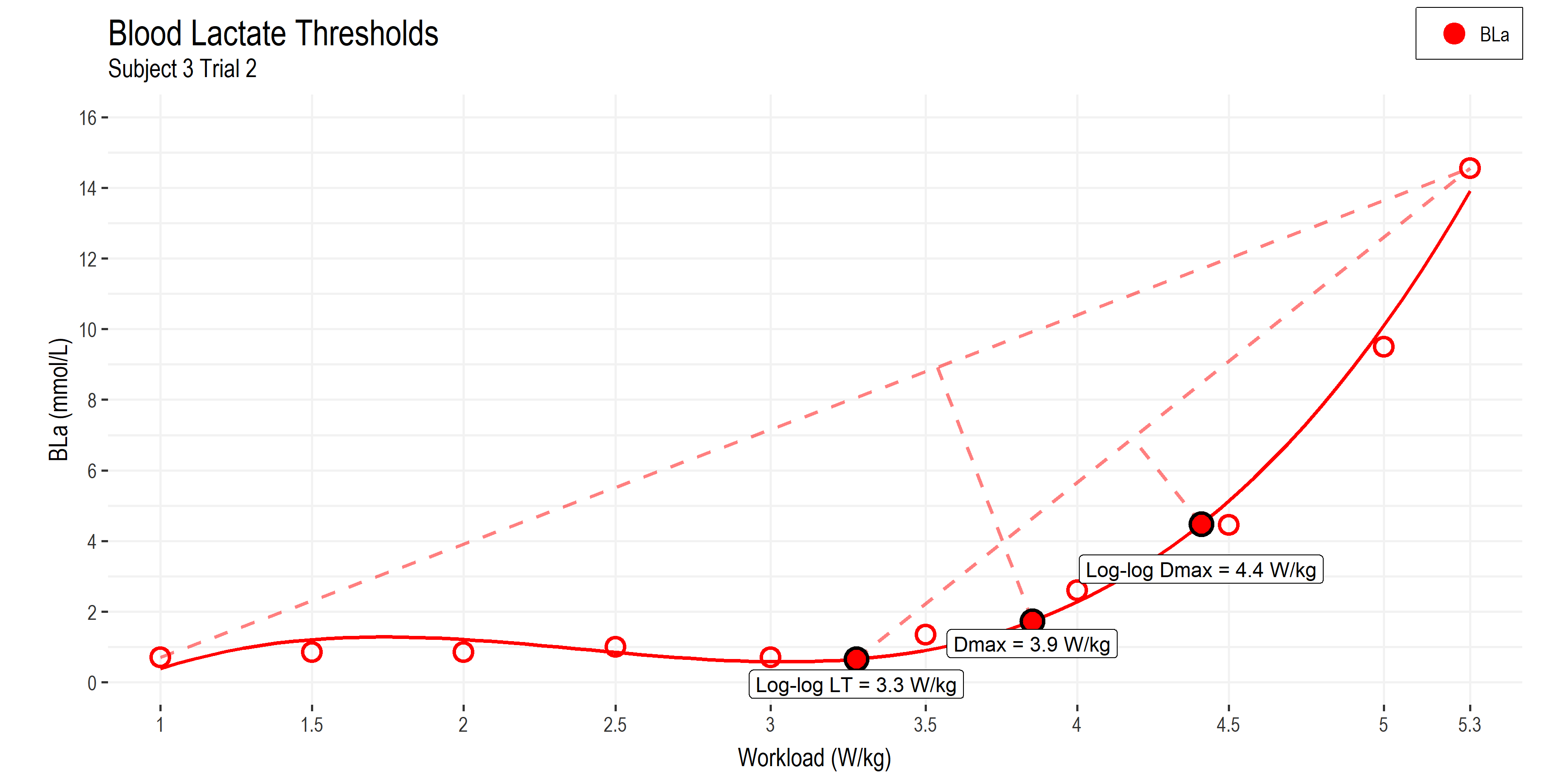
• Power (W/kg) is now on the x-axis.
• Blood lactate (BLa) on the y-axis, now with units from 0 to 16 mmol/L
• LogLog LT: method of estimating Lactate Threshold 1 (details below).
• Dmax: method of estimating Lactate Threshold 2.
• LogLog Dmax: a modified method of estimating Lactate Threshold 2 that may be more closely related to MLSS and CP than Dmax.

I’m using the well-established Dmax (distance max) method for deriving a breakpoint in the lactate curve. This finds the greatest perpendicular distance from the line connecting the first and last BLa data points, to the curve fitted to all the BLa data points with a 3rd order polynomial function. This method is related to maximum lactate steady state (MLSS) or lactate threshold 2, although the validity has been questioned and the agreement may underestimate MLSS and CP (Jamnick et al, 2020). The Dmax method finds a breakpoint at 3.9 W/kg for this athlete.

The second method I’m using is the log-log transform of BLa (not pictured) to derive the first breakpoint (LT1, at 3.3 W/kg) where BLa begins to increase logarithmically. From this, a modified Dmax method run from the log-log LT value to the peak BLa value. This log-log Dmax method has been shown to produce an LT2 estimate that is more closely related to MLSS and CP than the original Dmax method. This occurs at 4.4 W/kg for this athlete.

Determining lactate thresholds was the most straight forward for this exercise protocol, since classic lactate testing is done with a multi-stage assessment with similar work stage durations (3-10 minutes). But we can see that the breakpoints differ depending on the analysis method. ie. between 3.9 – 4.4 W/kg for LT2. So we have only started to narrow down a potential range for the physiological breakpoints to occur around.

---

Ventilatory Thresholds

Ventilatory thresholds are a bit more tricky to model for this protocol: Ventilatory threshold 1 (or gas exchange threshold; GET) and VT2 (or respiratory compensation point; RCP) are typically derived from a much shorter 8-12 minute incremental ramp test, where ventilation increases rapidly and usually in a predictable intensity-dependent manner. During a longer multi-stage assessment, ventilation will respond to the duration of work at each stage, as well as to intensity. So the typical analysis methods for breakpoint detection may not be as reliable.

• Pulmonary O2 uptake (VO2) on the x-axes.
• In the left-side chart, pulmonary CO2 expiration (VCO2) and Ventilation (VE) on the left and right y-axes.
• In the right-side chart, ventilatory equivalents (VE relative to VO2 and VCO2, respectively) are plotted on the y-axis.
• In both charts, a modeled stepwise function shows the workload (W/kg) at which the VO2 on the x-axis occurred. This is just a simple way to visualize and relate VO2 on the x-axis to power output for demarcating breakpoints.

I’m starting with the classic V-slope method for determining the gas exchange threshold (GET), by plotting the breakpoint in VCO2 (CO2 production, in purple on the left-side chart) relative to VO2 (O2 uptake on the x-axis). This point indicates a disproportionate rise in ‘non-metabolic’ CO2 production from the buffering of H+ produced from so-called ‘anaerobic’ or cytosolic glycolysis (Meyer et al, 2005). This breakpoint is found at 4.5 W/kg on the left-side chart for this athlete.

GET is related to, but not synonymous with VT1. VT1 is shown on the left-side chart with VE in blue reaching it’s first breakpoint relative to VO2 on the x-axis at 4.5 W/kg. And confirmed on the right-side chart with VE/VO2 in green reaching a minimum also at 4.5 W/kg.

The second ventilatory threshold (VT2) or respiratory compensation point (RCP) is found by looking for the deflection of VE relative to VCO2, which reflects the onset of exercise-induced hyperventilation stimulated by a number of factors related to exceeding metabolic homeostasis. We can look at the transformed VE/VCO2 in the right-side chart, in orange. This reaches a first breakpoint at 4.0 W/kg, which indicates the flattening of VE relative to VCO2 as VT1 (4.5 W/kg) is approached. Then the second breakpoint at 5.0 W/kg indicates a second disproportionate rise in VE. This is observed in VE vs VO2, in blue on the left-side chart, and equally in VE/VO2 (green) and VE/VCO2 (orange) on the right-side chart.

So our ventilatory thresholds are very consistent with each other for this athlete, with VT1 estimated around 4.0-4.5 W/kg, and VT2 estimated at 5.0 W/kg. Interestingly, however, these are slightly higher than the equivalent lactate thresholds for this athlete (LT1 ~3.3 W/kg, and LT2 3.9-4.4 W/kg). This could simply be a limitation of the algorithmic breakpoint detection method, or, as I suspect, a more intrinsic physiological relationship related to the duration of the assessment protocol. I can’t think of the precise mechanisms why ventilatory thresholds would be delayed compared to lactate breakpoints in a longer multi-stage test such as this, but maybe I’ll think of something and edit an answer in here. 🙂

With the traditional lactate and ventilatory thresholds taken care of, let’s turn our attention to some NIRS breakpoints measured by Moxy.

---

NIRS-derived Deoxygenation Breakpoints

The closest thing to an established method for analysing NIRS data for breakpoint detection comes from research using the traditional 8-12 minute incremental ramp test protocol that I mentioned above, for comparison to ventilatory thresholds. In this protocol, a simple double-linear breakpoint (piecewise or segmented linear regression) can be used to find the breakpoint in the NIRS signal. This is basically identical to the V-slope method for ventilatory thresholds which we used above. The NIRS breakpoint is typically described as occurring at the equivalent of VT2 or ‘deoxygenation-breakpoint’ (deoxy-BP).

(Keir et al, 2015)
• Here is a good example showing a direct comparison between ventilatory and NIRS breakpoints (HHb: deoxyhemoglobin; the deoxygenation component of the NIRS signal) in a ~14-minute incremental ramp test protocol.
• On the left side, ventilatory thresholds vs VO2 on the x-axis, with RCP (VT2) marked.
• On the right side, VO2 and HHb vs time on the x-axis, with the HHb-BP (deoxy-BP) marked.
• Inset table with pulmonary VO2 and power output (PO) breakpoints for multiple evaluation methods.
• Breakpoint lines indicate that RCP and HHb-BP both occur at ~ 3.5 L/min VO2, and the inset table shows power output is also similar at 270-275 W.

The protocol we are using is much longer, and uses constant workload stages rather than a continuous incremental ramp in power output, so I can’t use the exact method shown above. There is no consensus around how to determine relevant NIRS breakpoints from a longer duration multi-stage assessment protocol such as this. However, as I mentioned, the sport science community has proposed a few important signals to look at for manual interpretation.

Let’s first look at the time series SmO2 recordings from a few muscle sites of interest.

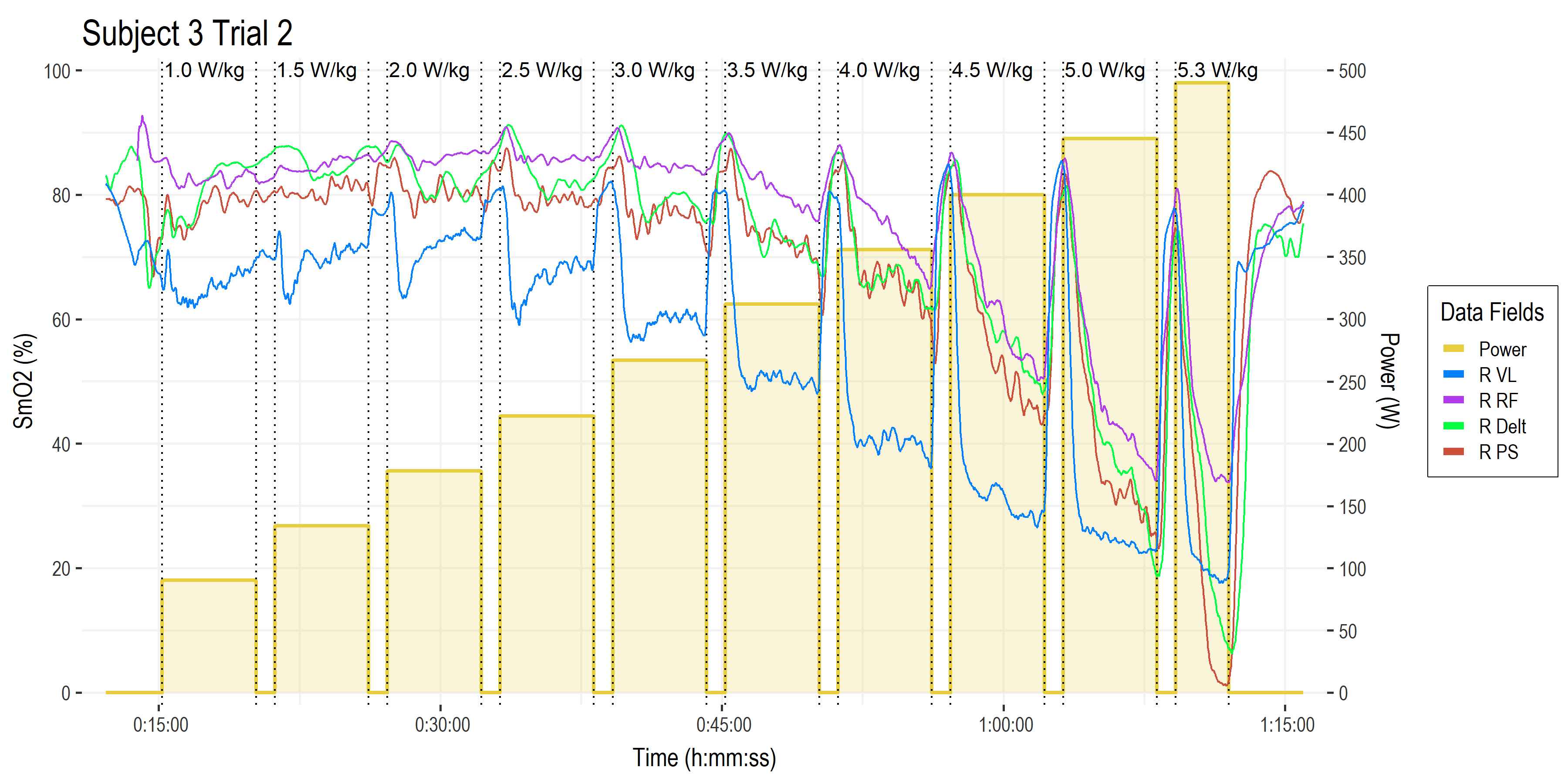
• Time on the x-axis.
• Power (W ) on the right-side y-axis, with bars showing work stage power targets and W/kg along the top.
• Muscle oxygen saturation (SmO2, %) on the left-side y-axis, with four muscles of interest shown from the right side of the body (left side not shown for clarity).
• Vastus lateralis of the quadricep muscle (blue). This is the primary locomotor muscle involved in cycling and most of the NIRS literature is on this muscle.
• Rectus femoris (purple), a secondary locomotor quadricep muscle more commonly evaluated in running.
• Deltoid shoulder muscle (green), which is an upper body stabilizer in the context of cycling that gives a picture of ‘systemic’ oxygenation status.
• Lumbar erector spinae or paraspinal muscles (brown), which are postural stabilizers, and incidentally show a much greater response than we had expected! (keep reading!) I have not yet encountered any literature with NIRS on paraspinal muscles during cycling exercise.

This gives us a good wholistic view on the response profiles of the various NIRS channels. What are we actually looking at? What are the relevant signals? The first thing we might notice is that the average value of each SmO2 channel stays high for the first few stages, then begins to decrease as workload increases. The VL in blue appears to be more linearly related to workload, while the other muscle sites show a more curvilinear response to increasing intensity.

The next thing we might notice is that the SmO2 line during each work stage itself begin to decline: the slope of SmO2 during the work intervals starts positive or flat, and become more and more negative at higher workloads.

We also might think those big re-saturation spikes during the recovery intervals are probably important – and they are – but I’ll have to save those analyses for another time. 🙂

Let’s start with these two parameters to investigate:

1. Work interval mean steady-state SmO2 value: the average value after SmO2 initially de-saturates and reaches a relative metabolic ‘steady-state’, ie. in the last 3-minutes or so of each 5-minute work stage.
   
2. Work interval steady-state SmO2 slope: the slope of SmO2 over time during that same steady state (last 3-minute) period of each work stage.

---

SmO2 Values Breakpoint Detection

We can start once again by transforming the plot to express SmO2 from each work stage on the y-axis, and stage workload on the x-axis. This gives us something comparable to the BLa and ventilation charts that we analysed, above.

• Power (W/kg) on the x-axis
• Each chart shows mean SmO2 (%) from the last 3-minutes of each 5-minute work stage.
• Top-left: vastus lateralis (blue).
• Top-right: rectus femoris (purple).
• Bottom-left: deltoid (green).
• Bottom-right: paraspinals (brown).

This certainly gives us a sense of the overall response profile from each muscle site. But how to we determine breakpoints? Why don’t we start with a double-linear or V-slope model, such as has been used for ventilation and the HHb-BP (deoxy-BP) during a ramp incremental test.

• As above; mean SmO2 (%) from vastus lateralis (blue), rectus femoris (purple), deltoid (green), and paraspinals (brown).
• Double-linear or piecewise linear regression to determine a single breakpoint from this simplified response profile from each work stage. To replicate the method used to detect ventilatory breakpoints.

When we fit the data to a double-linear model with a single breakpoint we get a reasonable first approximation for a deoxy-BP… at least, for three of the four muscles. The VL (blue) shows an early deflection that probably doesn’t represent loss of metabolic homeostasis at such a low workload (2.2 W/kg) for this highly trained athlete. But rather, these low-intensity work stages are probably acting to produce a warm-up effect, and we’re seeing a relative increase in blood flow and perfusion, which we might call an ‘oxygenation breakpoint’; oxy-BP.

RF (purple) shows the next breakpoint at 3.4 W/kg. Just about at 50% through the test protocol. This may be reasonable, based on how RF is recruited as a ‘secondary’ locomotor muscle at moderate workloads (Chin et al, 2011). But again, whether this equates to a systemic loss of homeostasis is questionable.

Although, we have to remember that local tissues might reach metabolic deflection points at different workloads based on relative recruitment and local disruptions to metabolic milieu. Maybe we should expect to see the locomotor muscles such as VL and RF reach their breakpoints earlier than systemic parameters of pulmonary ventilation and capillary blood lactate?

Speaking of which, the bottom two charts showing deltoid and paraspinals are interesting: They show closely related breakpoints at 4.2-4.3 W/kg, which are well within the range of the second lactate and ventilatory thresholds (3.9-5.0 W/kg).

However, if we look back at the raw data points, is the overall response best described by a double-linear model? Or would these two non-locomotor muscles be better described by a curvilinear model? Let’s use the Dmax model that we applied to the lactate curves, above, where we run a polynomial fit and look for the furthest distance to a line through the first and last values, and compare our results.

• As above; mean SmO2 (%) from vastus lateralis (blue), rectus femoris (purple), deltoid (green), and paraspinals (brown).
• Dmax method on polynomial curve fitting, to determine a single breakpoint from this simplified response profile from each work stage. To replicate one of the common methods used to detect lactate thresholds.

These non-linear models do appear to better fit the data, however when I see a nearly symmetrical curvilinear response profile like these, I have to ask: why are we trying to find the corner of a circle? The Dmax models for RF, Delt, and PS basically just return the middle point along a quadrant of a circle. But that’s probably a discussion for another time.

These breakpoints are feeling somewhat arbitrary to me, so let’s look at the second parameter: the slope of SmO2 during each work stage.

---

SmO2 Slope Breakpoint Detection

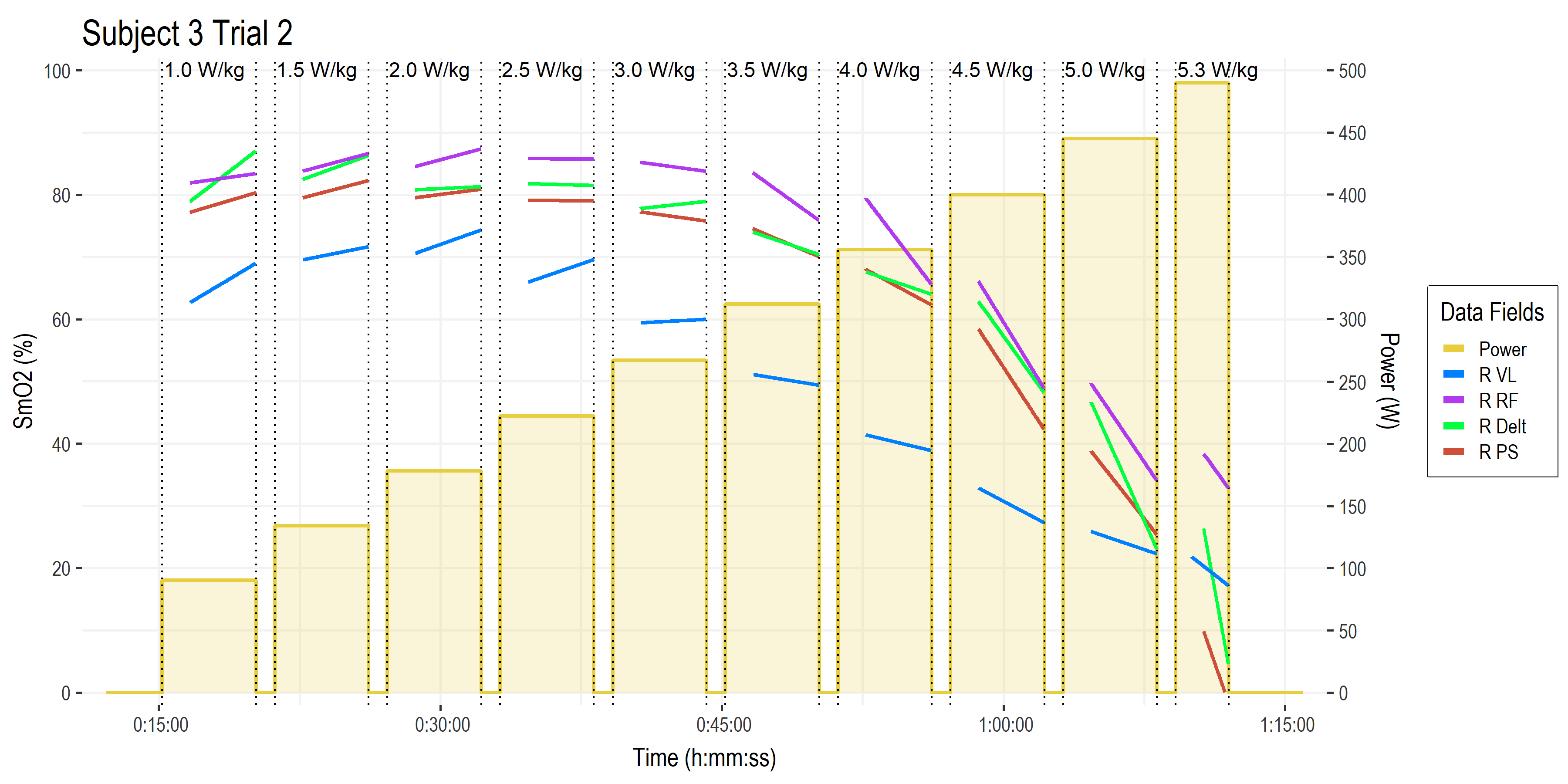
• Time on the x-axis.
• Power (W ) on the right-side y-axis, with bars showing work stage power targets and W/kg along the top.
• Muscle oxygen saturation (SmO2, %) on the left-side y-axis
• Now we are just looking at the linear slope plotted through the last 3-ish minutes of each work stage, describing the ‘steady-state’ kinetics after onset kinetics have reached an equilibrium within the first ~90-seconds.

What we are interested in here is whether the slope is meaningfully positive, negative, or neutral. SmO2 is a relatively scaled index of the balance of oxygen delivery (blood flow, O2 perfusion and diffusion) and oxygen utilization (muscle O2 uptake; mVO2).

When O2 delivery is greater than O2 uptake, SmO2 will be increasing (positive slope). We can see this occurring during the lower intensity work stages, where the athlete experiences a ‘warm-up’ effect, where blood flow increases to the working muscles, delivering more O2 relative to the rate of utilization to produce power.

When O2 uptake is greater than O2 delivery, SmO2 will be decreasing (negative slope). We see this occurring during the higher intensity stages. This would typically be interpreted to indicate the athlete is not able to reach metabolic equilibrium, ie. they are not able to deliver O2 at the rate required to meet the rate utilization to produce power.

• Transformed back to power on the x-axis (W/kg)
• SmO2 slope (SmO2 %/min) from vastus lateralis (blue), rectus femoris (purple), deltoid (green), and paraspinals (brown), during each work stage.
• Zero slope highlighted at the dotted line.
• Note each subplot has it’s own y-axis scaling

With the SmO2 slopes plotted vs workload on the x-axis, we can see where the work stage slopes become negative (dotted line at zero slope). So do these zero-crossing points represent a transition from sustainable to non-sustainable workload? ie. critical power or maximum metabolic steady state?

I don’t think it’s quite this simple: because we are not just observing responses to intensity or workload alone: we have a dose-dependency response, where the dose is a product not just of the intensity, but also the duration of work at that intensity.

We are only allowing a 5-minute interval for all of these interrelated metabolic processes to reach an ‘equilibrium’ at each target workload. However, the responses we observe after 5 minutes may continue to shift – the metabolic intensity would change – if we continued to work at the same workload.

This is especially true around the heavy intensity domain, at the mid-range of workloads in this protocol: At these intensities, substrate oxidation (fatty acids and carbohydrates) shift dynamically, and metabolic homeostasis is delayed (a gradual shift continues) at least until the 6th minute of constant workload exercise (Colosio et al, 2020; Colosio et al, 2021).

This would suggest that, while the apparent 5-minute slope might appear negative, given longer observation at the same constant workload, the NIRS signals might reach a delayed equilibrium and subsequently exhibit ‘steady state’ or ‘zero-slope’ behaviour.

So possibly, a margin of error should be allowed around the zero-slope line to predict a ‘meaningful’ crossing of zero into a negative slope that would truly stay negative until task intolerance, indicating the intensity is above the maximum metabolic steady state? Somewhat arbitrarily, why don’t we say -2% SmO2/min? This is based on the manufacturer’s guidelines of a meaningful change (equivalency interval) of ±5%, which gives us a range of 10% over a 5-minute interval (discounting onset kinetics) to show a meaningful change = -2% SmO2/min. Very arbitrary, indeed…

Let’s otherwise stick to familiar territory for modeling these slope responses, and we’ll fit a 3rd order polynomial regression line through the slope values.

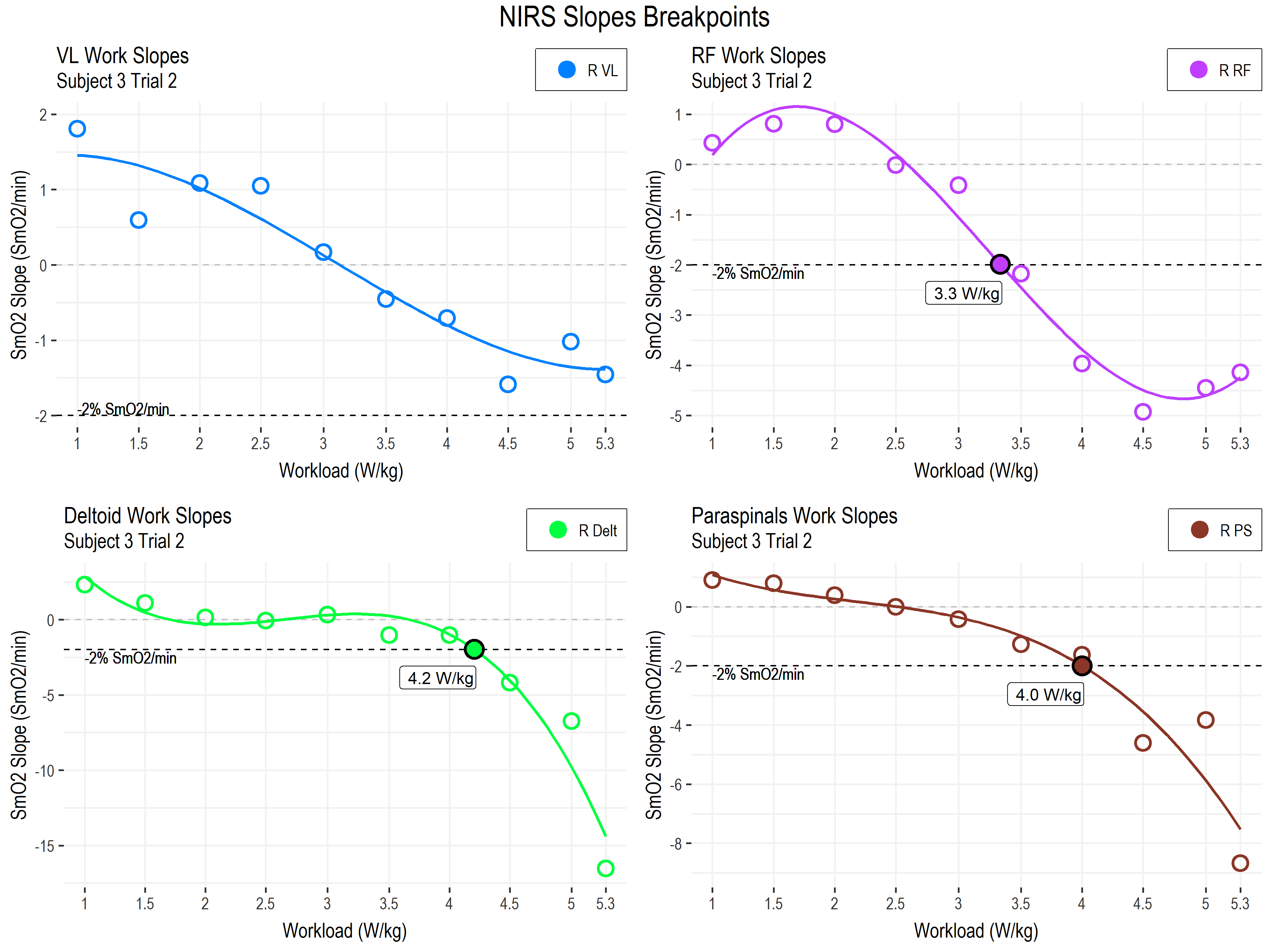
• As above; SmO2 slope (SmO2 %/min) from vastus lateralis (blue), rectus femoris (purple), deltoid (green), and paraspinals (brown), during each work stage.
• -2 % SmO2/min slope highlighted at the dotted line.
• Note each subplot has it’s own y-axis scaling

The first thing we can see is the heterogeneity of response profiles across the different muscle sites. This is probably to be expected, since we are looking at a combination of primary locomotor, secondary locomotor, and non-locomotor muscles.

The breakpoints in the deltoid and paraspinals, at 4.0-4.2 W/kg, are within the range of the second lactate and ventilatory thresholds (3.9-5.0 W/kg). And the RF breakpoint, maybe coincidentally, agrees with LT1 at 3.3 W/kg.

The VL slopes do not appear to be meaningfully different from zero, at least in our arbitrary model here. We have also seen this across our other subjects. For this muscle, the absolute values may be more important than the slope during work stages.

The deltoid and paraspinals (non-locomotor muscles involved in postural and upper body stabilization) however, demonstrate a sudden and steep breakpoint into negative slope. This may be the most insightful trend, and may represent the combined effects of a local and systemic shift to non-sustainable metabolism:

Locally, these muscles are themselves working to stabilize the trunk, pelvis, and upper body, in order to resist the internal forces from the legs pushing on the pedals. So we should expect metabolic work to increase at these muscles as well as at the locomotor muscles. We might also expect intramuscular pressures from contraction forces to rise, until a certain point where the pressure of muscle contraction actually squeezes the small blood vessels and begins to limit blood flow and O2 delivery.

Systemically, the body will be trying to redistribute it’s total blood volume toward the tissues with the highest metabolic demand. During cycling, this is of course the legs. So the locomotor muscles will experience vasodilation to increase blood flow, while much of the rest of the body will experience vasoconstriction, to restrict blood flow. With a limited cardiac output and blood volume to distribute across tissues with competing metabolic demands, the sharply negative slopes at the deltoid and paraspinal muscles could represent a necessary restriction of blood flow to these tissues at higher intensities, in order to maintain the required O2 supply to the legs.

So we have a fair physiological rationale for using SmO2 slope for non-primary locomotor muscles. And we have decent agreement between lactate, ventilatory, and SmO2 slope breakpoints in this single subject. What about wider agreement in a larger sample group?

---

Correlation and Agreement between Breakpoints

In our lab, we have looked at all of these breakpoints in a group of 21 male and female trained cyclists, and compared the correlation and agreement among them. I can show some preliminary results, but I should really stress that these are only directional, and should not be taken as conclusive. These analyses and results are likely to change.

Blog posts are meant for speculation. Forming conclusions should wait for peer-reviewed research with more rigorous analysis methods. 🙂

Briefly, the correlation coefficient (r or R) relates to how closely two measures are linearly related; that is, as one measurement increases, how closely does the other measurement either increase (for positive R) or decrease (negative R). A greater negative or positive value closer to -1 or 1 indicates a stronger proportional relationship. We can model this with simple linear regression, comparing, for example, Power at log-log Dmax LT2 vs Power at VT2, from the methods we described above.

Agreement describes by how much the two measurements tend to differ. We will use Bland-Altman plots to describe the limits of agreement (LoA; or 95% confidence interval; CI) as an estimate of where 95% of the population differences are expected to fall within. Since the two measures have the same units (W/kg) we can describe the limits agreement in relation to an a priori ‘meaningful limit’. So in our case, we could say that we want 95% of the values to agree within ± 0.5 W/kg, or no more than one stage difference.

We hope to find high correlation and low limits of agreement between our breakpoint methods. First, let’s compare our lactate and ventilatory threshold methods to get a baseline for systemic thresholds, and to understand what we are looking at.

• We are comparing power at LT2 using the log-log Dmax method (LogLogDmaxPower), against power at VT2 using the V-slope method (ExpertVT2), both described above. Both measurements are in W/kg.
• Dots represent individual trials performed by subjects.

• On the left-side chart: linear regression and correlation.
• Dotted line of identity, where y = x would describe a perfect relationship between measurements.
• Solid black modeled regression line with slope of 1.05 and high R and R^2 values describe a significant (p < 0.05) strong, positive proportional relationship between the two measurements.

• On the right-side chart: Bland-Altman plot with 95% CI limits of agreement.
• Solid horizontal line at the mean bias, describing the mean difference between measurements; closer to zero is better.
• Dashed horizontal lines marking the upper and lower 95% CI LoA, containing 95% of the sample data. We set our a priori meaningful limits to ± 0.5 W/kg, and we can see the LoA here are close to that.

This is a good benchmark, as we would hope to see strong correlation and agreement between systemic thresholds measured from different parameters within the same assessment trial.

To cut to the chase, the NIRS breakpoints with the strongest preliminary results in our sample group was actually from the paraspinals location! All three breakpoint detection methods showed good correlation (r > 0.8) and good to fair limits of agreement (< ± 0.6 W/kg) with either lactate or ventilatory thresholds.

This was unexpected. We originally thought paraspinals or erector spinae muscles might reveal bilateral differences related to biomechanical asymmetry and injury history, or injury risk. We did not think they would show such an apparently robust relationship to exercise intensity.

---

Paraspinal Muscle Involvement in Cycling

To briefly speculate on this relationship, we already talked about how these postural stabilizers are metabolically involved during higher exercise intensities. And anecdotally, we have probably all experienced some back discomfort during or after long and hard cycling sessions. So maybe it should not have been such a surprise that they appear to be working hard to stabilize the trunk and pelvis, to give the legs a stable base of support off of which to push on the pedals.

Methodologically, the PS may be a good site for evaluation with NIRS during cycling, as they tend to have lower adipose tissue thickness in both male and female subjects. They are predominantly in an extended position under tension during cycling, in a position where the tissues don’t move much under the sensors. Muscle fiber composition of the paraspinals might also be preferable, as they tend to be highly aerobic (type I slow twitch) fiber typology (Jørgensen, 1997). And the much smaller muscle mass compared to the quadriceps may allow greater relative penetration through the muscle interior by the optical NIRS signal.

• Our experimental set-up for Moxys on paraspinals.
Location was on the bilateral mid muscle belly approximately at the level of L3 vertebrae. Moxy sensors were taped directly to the skin as pictured. Light shielding was typically provided by subject’s cycling bib shorts, or for subjects such as this athlete, additional opaque black tape was placed overtop the sensors.

I can report, it’s a bit tough to place these on yourself the first time for self-testing, but once you get the trick it’s not bad!

---

The strongest two relationships between any NIRS breakpoint (both are from PS) and systemic thresholds are visualized below. One was using the Dmax method on PS SmO2 values, the other was using the polynomial method on PS slopes. There were other interesting interrelationships between NIRS-derived breakpoint methods that I won’t get into here.

• Power at LT2 using the Dmax method (DmaxPower) compared to power at NIRS Deoxy-BP using the Dmax method on paraspinals (PSDmaxPower). Both measurements are in W/kg.

• Linear regression shows a strong significant correlation and positive proportional relationship, and limits of agreement are within our ± 0.5 W/kg meaningful range.

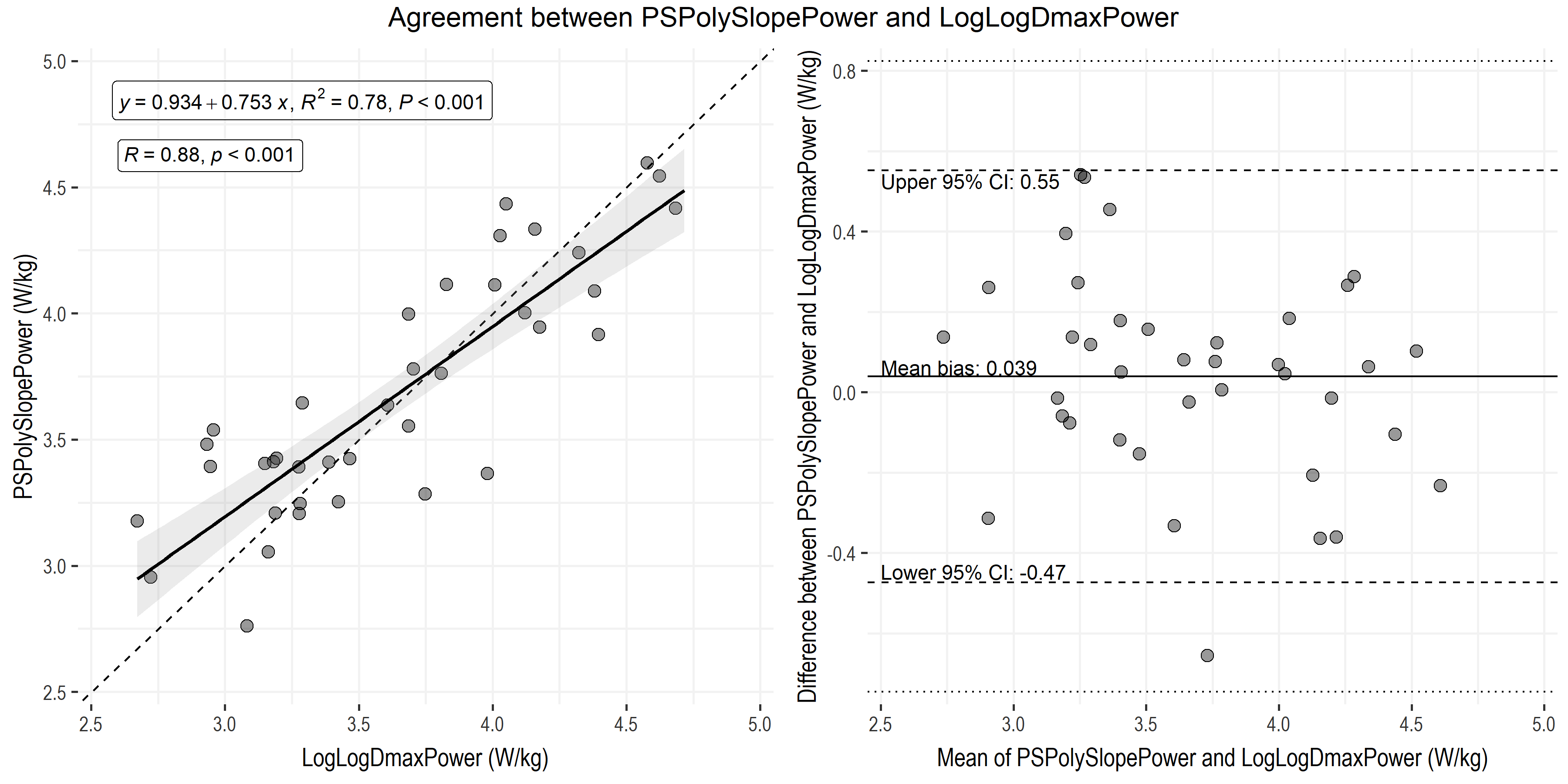
• Power at LT2 using the LogLogDmax method (LogLogDmaxPower) compared to power at NIRS Deoxy-BP using the polynomial method on slope of paraspinals (PSPolySlopePower). Both measurements are in W/kg.

• Linear regression shows a strong significant correlation and positive proportional relationship, and limits of agreement are within our ± 0.5 W/kg meaningful range.

---

Conclusions, or Lessons from the Process

Having gone through this exploratory process, what do these preliminary results suggest? There have been many debates in recent years how closely NIRS-derived breakpoints agree or don’t agree with, can or cannot be used to predict traditional systemic thresholds, and should or should not be used for training prescription. I don’t think I care to add much to either side of that debate for now.

I do think what we are seeing, and the lessons I am taking away from this process so far, are that:

1. We should expect varied responses across locomotor and non-locomotor muscles between individuals, and how the accumulation of local, peripheral responses contribute to the observed systemic responses. Variance between thresholds does not necessarily imply the absence of an underlying relationship, but does imply meaningful variability in the nature of those relationships at the particular moment of evaluation. Which, if understood systematically, can be exploited to optimize training prescription and improve performances for individual athletes.
   
2. Breakpoint detection is difficult to algorithmically define for even the most established parameters, supporting the growing understanding that these thresholds aren’t hard and fast physiological light-switches, but describe transition zones between general metabolic responses to varying intensities. Maybe we should be using algorithmic methods to describe the overall shape of a given response profile, but resist the urge to oversimplify that response profile to a single point of change? Maybe our training should focus on eliciting and maintaining a desired response profile, which can be monitored and adjusted in real-time?

The next generation approach to metabolic profiling and training prescription will almost certainly not include breakpoints or thresholds at all, and will use more flexible methods of describing continuous physiological response profiles in real-time. There are already devices, tools, and services that at least claim to support this approach.

I do think a systematic, algorithmic, machine learning, AI.. (whatever buzzword you want to use) approach should be part of the goal of standardizing interpretation of metabolic data. Our brains are good – often too good – at picking out patterns automatically and subconsciously. I think that by defining the rules which our brains are already using, we will be able to better understand the real physiological relationships for an individual athlete, and improve how we can apply insights to that individual athlete’s training.